econometron.Models.dynamicsge.linear_dsge

• class in the econometron.Models.dynamicsge module

Overview

A Dynamic Stochastic General Equilibrium (DSGE) model describes the decisions of households, firms, and policymakers under uncertainty, subject to market-clearing conditions. A linear DSGE model is the first-order Taylor approximation of the model’s nonlinear equilibrium conditions around a deterministic steady state. The linear_dsge class in econometron.Models.dynamicsge allows specification, solution, and analysis of linear and log-linear DSGE models.

Linearization

Given a nonlinear equilibrium system:

let be the steady state. The linearized system is obtained by a first-order expansion in deviations:

Example (levels) If:

then, around :

• Units: original scale
• Use case: variables can be negative (e.g., interest rate gaps)

Log-Linearization

For positive variables, define the log-deviation:

Apply the Taylor expansion to the logged equations.

Example (logs) If:

then:

• Units: percentage deviations from steady state
• Use case: real, strictly positive variables (e.g., output, capital)

In Practice

• Linearization: use for rates, spreads, gaps.
• Log-linearization: use for real quantities.

---

class linear_dsge capabilities

• Parse string-based equations
• Compute steady states
• Linearize or log-linearize
• Solve RE systems (Klein(2000))
• Simulate and compute IRFs
• Support for analytical and numerical steady-state and derivative computation

Class Definition

from econometron.Models.dynamicsge import linear_dsge

lineardsge=linear_dsge(
                 equations=list[str],
                 variables=list[str],
                 exo_states=list[str],
                 endo_states=list[str],
                 parameters=dict[str, float],
                 approximation=str,
                 normalize=bool,
                 shocks=list[str])

Parameters

Name	Type	Description	Default
equations	list[str]	Model equations as strings, must include = and time subscripts (_t, _tp1, _tm1).	None
variables	list[str]	Variable names (e.g., ['A', 'K', 'C']).	None
exo_states	list[str]	Exogenous state variables.	None
endo_states	list[str]	Endogenous state variables.	None
parameters	dict	Model parameters, e.g., {'sigma': 1.5}.	None
approximation	str	'linear' or 'log_linear'.	'linear'
normalize	dict	Steady-state normalization values.	{}
shocks	list[str]	Shock variable names.	None

Attributes

Attribute	Type	Description
equations_list	list[str]	Provided equations.
variables	list[str]	All model variables.
exo_states	list[str]	Exogenous state variables.
endo_states	list[str]	Endogenous state variables.
states	list[str]	Combined exogenous + endogenous states.
controls	list[str]	Variables not in states.
parameters	dict	Model parameters dictionary.
approximation	str	Approximation type.
normalize	dict	Normalization values.
shocks	list[str]	Shock variables.
n_vars, n_equations, n_states, n_exo_states, n_endo_states, n_controls	int	Model dimension counts.
steady_state	pd.Series	Steady-state values.
A, B, C	np.ndarray	Jacobian matrices.
f, p	np.ndarray	Policy and state transition matrices.
irfs	dict[pd.DataFrame]	Impulse response functions.
simulated	pd.DataFrame	Simulated data.
initial_guess	numpy array	Initial guess for steady state.

Methods

1 - validate_entries()

• Purpose: Validates inputs during initialization. It checks:

  • Non-empty list of equations containing =.
  • Non-empty variables list without duplicates.
  • Non-empty parameters dictionary.
  • Correct data types for states and shocks.

• Returns:

  • True if valid; otherwise raises ValueError or issues warnings.

2 - set_new_parameters(params)

• Purpose:

  Updates model parameters (self.parameters).

• Returns:

  Prints updated parameters or warns if update fails.

3 - set_initial_guess(initial_guess)

• Purpose:

  Sets initial guess for steady-state computation.

  • If approximation="linear", the exogenous shock is set to 0.
  • If approximation="log-linear", the exogenous shock is set to 1.
  • You can use normalize = {var: value} to assign a specific value to a given variable.Generally, you don’t need to provide this unless required.
  • If set_initial_guess and guess is not specified, it defaults to an array of ones with length equal to the number of endogenous variables.

• Returns:

  • Stores as np.array could be checked by :
    • Example python lineardsge.initial_guess
  • Raises ValueError if size/type mismatch.

4 - compute_ss(guess=None, method='fsolve', options=None)

purpose

• Computes steady state via numerical optimization,currently suppoting fsolve. if user didn't specify the initial via guess or set_initial_guess(),it will default to an array of ones with the same length as the endogenous variables.

• Parameters:

  • guess – Initial guess (defaults to ones).
  • method – Only 'fsolve' supported.
  • options – Optimizer options.

• Returns:

  • pd.Series steady-state values

5 - approximate(method=None, debug=False)

• Purpose:

  • Approximates the Rational Expectations (RE) model around its steady state using either analytical or numerical Jacobians.
  • Uses _Analytical_jacobians (symbolic, more stable and parsimonious) or _Numerical_jacobians.
  • Both functions internally call _reorder_variables, which reorders variables in the sequence: exo_states → endo_states → controls.
  • Stores Jacobians as self.A, self.B, self.C.
  • Once approximated,The model attribute approximated = True and the model can be solved using the Jacobians.
  • Note : This method must be called after compute_ss(). If approximate() is called when approximated = True, a Warning is raised to notify that the model is already approximated; users should only call this method once after computing the steady state.

• Parameters

  • method : analytical or numerical default : analytical
  • debug : bool, optional
    • If True, enables debug mode for more verbose output.

• Returnstuple: (A, B, C)

  • A – Jacobian matrix associated with expectations
  • B – Jacobian matrix associated with current endogenous variables
  • C – Jacobian matrix associated with exogenous shocks

6 - solve_RE_model(Parameters=None, debug=False)

• Purpose:

  Solves the Rational Expectations (RE) model of the form

  using Klein’s method (generalized Schur decomposition - Solab.m 2000).

  • If Parameters are provided, the Jacobians are recomputed analytically.
  • Otherwise, it uses the already stored approximated Jacobians.
  • The solution is stored in self.f (policy function) and self.p (state transition function).
  • This function can be used once The model is approximated.

• Parameters

  • Parameters (dict, optional): Model parameters to override.
  • debug (bool, optional): If True, enables debug mode for more verbose output.

• Returns

  tuple: (F, P)

  • F – Control function, mapping states to controls:

  • P – State transition function, governing the law of motion:

7 - _compute_irfs(T=51, t0=1, shocks=None, center=True, normalize=True)

• Purpose:

  • Computes impulse response functions (IRFs) for a DSGE model, adjusted to match the behavior of the impulse method. IRFs describe the dynamic response of model variables to exogenous shocks.
  • Simulates the model’s response to specified shocks over T periods.
  • Stores results in self.irfs as a dictionary of DataFrames, with each key corresponding to a shock and its associated IRFs.
  • Ensures compatibility with log-linear or linear approximations, with options to center (return deviations) or normalize (divide by steady state).

• Parameters:

  • T (int, optional): Number of periods for IRF computation (default: 51).
  • t0 (int, optional): Time period when shocks are applied (default: 1).
  • shocks (dict, optional): Dictionary of shock names and magnitudes. If None, applies a 0.01 shock to each defined shock (default: None).
  • center (bool, optional): If True, returns deviations from steady state; if False, returns levels or log levels (default: True).
  • normalize (bool, optional): If True, normalizes linear approximation IRFs by steady state values (default: True).

• Returns:

  • dict: Dictionary where keys are shock names and values are pd.DataFrame objects containing IRFs for states, controls, and the shock itself.

  • Notes:

    • Requires f (policy function) and p (state transition function) to be defined.
    • Raises ValueError if model matrices or shocks are undefined.
    • Warns if normalization is requested but steady state contains zeros, setting normalize to False.

8 - plot_irfs(shock_names=None, T=41, scale=100, figsize=(12, 4), lw=5, alpha=0.5, title_prefix="IRF", ylabel="Percentage Deviation")

• Purpose:

  • Compute impulse Responses via _compute_irfs() which are stored in self.irfs.

  • Plots impulse response functions (IRFs) for specified shocks, with separate subplots for the corresponding exogenous state and other variables.

  • Generates a two-panel plot for each shock: one for the exogenous state, exo_states, and one for all other variables (states and controls).

  • Scales IRF values for better visualization and allows customization of plot aesthetics.

• Parameters:

  • shock_names (list, optional): List of shocks to plot. If None, plots all shocks in self.irfs (default: None).
  • T (int, optional): Number of periods for IRF computation if not already computed (default: 41).
  • scale (float, optional): Scaling factor for IRF values (default: 100).
  • figsize (tuple, optional): Figure size as (width, height) in inches (default: (12, 4)).
  • lw (float, optional): Line width for plots (default: 5).
  • alpha (float, optional): Line transparency (default: 0.5).
  • title_prefix (str, optional): Prefix for subplot titles (default: "IRF").
  • ylabel (str, optional): Y-axis label (default: "Percentage Deviation").

• Returns:

  • None: Displays the plots for each shock. Notes:
    • Raises ValueError if self.irfs is empty, not a dictionary, or if specified shocks/columns are missing.
    • Automatically adjusts y-axis limits for clarity.

9 - simulate(T=51, drop_first=300, covariance_matrix=None, seed=None, center=True, normalize=True)

• Purpose:

  • Simulates the DSGE model dynamics over T periods, adjusted to match the behavior of stoch_sim. Generates stochastic paths for states and controls driven by exogenous shocks.
  • Discards drop_first initial periods to eliminate transient dynamics.
  • Supports custom covariance matrices for shocks or defaults to a diagonal matrix based on shock variances.
  • Stores results in self.simulated as a DataFrame.

• Parameters:

  • T (int, optional): Number of periods to simulate (default: 51).
  • drop_first (int, optional): Number of initial periods to discard (default: 300).
  • covariance_matrix (array-like, optional): Covariance matrix for shocks (n_shocks x n_shocks). If None, uses a diagonal matrix with variances of 0.01² (default: None).
  • seed (int, optional): Random seed for reproducibility (default: None).
  • center (bool, optional): If True, returns deviations; if False, returns levels or log levels (default: True).
  • normalize (bool, optional): If True, normalizes linear approximation simulations by steady state (default: True).

• Returns:

  • pd.DataFrame: DataFrame containing simulated shocks and variables (states and controls).

  • Notes:

    • Requires self.f and self.p to be defined (model must be solved).
    • Raises ValueError if model matrices are undefined or covariance matrix has incorrect dimensions.
    • Warns if normalization is requested but steady state contains zeros, setting normalize to False.

10 - simulations(title="The Model Simulation", figsize=(12, 8), save_path=None)

• Purpose:

  • Plots the simulated data from simulate, with exogenous states in separate subplots and endogenous variables (states and controls) together in one subplot.

  • Creates a multi-panel figure where each exogenous state has its own subplot, and all endogenous variables are plotted together.

  • Allows saving the plot to a file or displaying it.

Parameters:

• title (str, optional): Title of the plot (default: "The Model Simulation").

• figsize (tuple, optional): Figure size as (width, height) in inches (default: (12, 8)).

• save_path (str, optional): File path to save the plot (e.g., 'plot.png'). If None, displays the plot (default: None).

• Returns:

  • None: Displays or saves the plot.
  • Notes:
    • Requires self.simulated to be a pd.DataFrame from a prior call to simulate.
    • Raises ValueError if self.simulated is not defined or no exogenous/endogenous variables are found.
    • Automatically adjusts layout to accommodate the title and subplots.

Usage Example – RBC Model

1 We Start By importing The class linear_dsge from the econometron.Models.dynamicsge module.

from econometron.Models.dynamicsge import linear_dsge

2 We Define The Model Equations as Follow ,specify all the variables, the exogenous , endogenous states and shocks along with the parameters.

equations = [
    "-C_t**(-sigma) + beta * C_tp1**(-sigma) * (alpha * A_tp1 * K_tp1**(alpha-1) + 1 - delta) = 0",
    "C_t + K_tp1 - A_t * K_t**alpha - (1 - delta) * K_t = 0",
    "-log(A_tp1) + rho_a * log(A_t) + epsilon = 0",
]
variables = ['A', 'K', 'C']
exo_states = ['A']
endo_states = ['K']
shocks = ['epsilon']
parameters = {
    'sigma': 1.5,
    'beta': 0.99,
    'alpha': 0.35,
    'delta': 0.025,
    'rho_a': 0.9,
}
RBC = linear_dsge(
    equations=equations,
    variables=variables,
    exo_states=exo_states,
    endo_states=endo_states,
    shocks=shocks,
    parameters=parameters,
    approximation='log_linear',
    normalize={'A': 1}
)

3 Once our Model RBC is defined, we can proceed with the following steps: we begin by set our initial guess for the computation of the steady-state. Since we have only 1 exo_state and using a simple guess, we can do:

RBC.set_initial_guess([1, 1])

RBC.compute_ss(method='fsolve', options={'xtol': 1e-8})

    Steady-state residuals: [-1.77851329e-13  9.03721542e-14 -1.00000000e-02]
    Warning: Large steady-state residuals detected.
    
    A     1.000000
    K    34.398226
    C     2.589794
    dtype: float64

4 Approximating The model around its steady state

RBC.approximate(method='analytical')

    (array([[-8.33790428e-03,  1.57555735e-04,  1.38972249e-01],
            [ 0.00000000e+00, -1.00000000e+00,  0.00000000e+00],
            [ 1.00000000e+00,  0.00000000e+00,  0.00000000e+00]]),
     array([[ 0.        ,  0.        ,  0.13897225],
            [-3.44974994, -1.01010101,  1.        ],
            [ 0.9       ,  0.        ,  0.        ]]),
     array([[0.],
            [0.],
            [1.]]))

5 Solving The model :

RBC.solve_RE_model()
print("Policy Function (f):\n", RBC.f)
print("State Transition (p):\n", RBC.p)

    Policy Function (f):
     [[0.59492193 0.03861978]]
    State Transition (p):
     [[0.9        0.        ]
     [2.85482802 0.97148123]]

6 Plotting Impulse Responses

RBC.plot_irfs()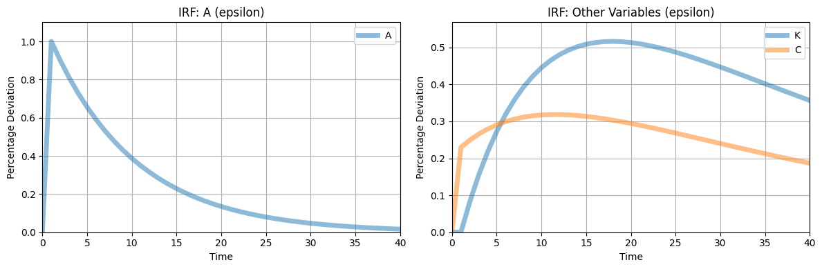

7 Simulations

RBC.simulate(T=51, drop_first=10)

8 Plotting The simulations

RBC.simulations()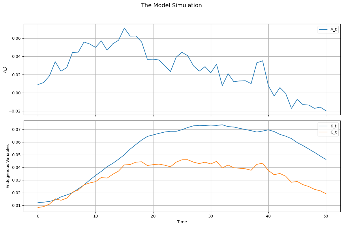

Notes

• Equation Syntax – Must use time subscripts (_t, _tp1).
• Log-Linear Approximation – Requires non-zero steady-state values.
• Shocks – If omitted, model is deterministic.
• Normalization – Overrides steady-state values for log-linear models.

Limitations

• Only 'fsolve' supported for steady states.